Load bounding box COCO annotations into ethology

Load bounding box annotations in COCO format as an ethology dataset and inspect it using ethology and movement utilities.

Imports

import os
from pathlib import Path

import matplotlib.pyplot as plt
import numpy as np
import pooch
import xarray as xr
from movement.io import save_bboxes
from movement.plots import plot_occupancy
from movement.roi import PolygonOfInterest

from ethology.io.annotations import load_bboxes

# For interactive plots: install ipympl with `pip install ipympl` and uncomment
# the following line in your notebook
# %matplotlib widget

Download dataset

For this example, we will use the dataset from the UAS Imagery of Migratory Waterfowl at New Mexico Wildlife Refuges. This dataset is part of the Drones For Ducks project that aims to develop an efficient method to count and identify species of migratory waterfowl at wildlife refuges across New Mexico.

The dataset is made up of a set of drone images and corresponding bounding box annotations. Annotations are provided by both expert annotators and volunteers.

Since the dataset is not very large, we can download it as a zip file directly from the URL provided in the dataset webpage. We use the pooch library to download it to the .ethology cache directory.

# Source of the dataset
data_source = {
    "url": "https://storage.googleapis.com/public-datasets-lila/uas-imagery-of-migratory-waterfowl/uas-imagery-of-migratory-waterfowl.20240220.zip",
    "hash": "c5b8dfc5a87ef625770ac8f22335dc9eb8a67688b610490a029dae81815a9896",
}

# Define cache directory
ethology_cache = Path.home() / ".ethology"
ethology_cache.mkdir(exist_ok=True)

# Download the dataset to the cache directory
extracted_files = pooch.retrieve(
    url=data_source["url"],
    known_hash=data_source["hash"],
    fname="waterfowl_dataset.zip",
    path=ethology_cache,
    processor=pooch.Unzip(extract_dir=ethology_cache),
)

data_dir = ethology_cache / "uas-imagery-of-migratory-waterfowl"

For this example, we will focus on the annotations labelled by the experts.

annotations_file = (
    data_dir / "experts" / "20230331_dronesforducks_expert_refined.json"
)

Load annotations as an ethology dataset

We can use the ethology.io.annotations.load_bboxes.from_files() function to load the COCO file with the expert annotations as an ethology dataset.

ds = load_bboxes.from_files(annotations_file, format="COCO")

print(ds)
print(ds.sizes)

<xarray.Dataset> Size: 353kB
Dimensions:      (image_id: 12, space: 2, id: 722)
Coordinates:
  * image_id     (image_id) int64 96B 0 1 2 3 4 5 6 7 8 9 10 11
  * space        (space) <U1 8B 'x' 'y'
  * id           (id) int64 6kB 0 1 2 3 4 5 6 7 ... 715 716 717 718 719 720 721
Data variables:
    position     (image_id, space, id) float64 139kB 4.493e+03 3.49e+03 ... nan
    shape        (image_id, space, id) float64 139kB 95.0 43.0 49.0 ... nan nan
    image_shape  (image_id, space) int64 192B 5472 3648 5472 ... 3648 5472 3648
    category     (image_id, id) int64 69kB 1 4 3 2 3 3 1 ... -1 -1 -1 -1 -1 -1
Attributes: (5)
Frozen({'image_id': 12, 'space': 2, 'id': 722})

We can see that the expert annotations consist of 2D bounding boxes, defined for 12 images, with each image having a maximum of 722 annotations. The position and shape arrays are padded with NaN for the images in which there are less annotations than the maximum. The category array is padded with -1.

Note that in this case a single annotation ID does not represent the same individual across images; it just represents an arbitrary ID assigned to each bounding box per image.

We can also see from the dataset description that it includes five attributes. These are stored under the attrs dictionary. We can inspect the content of the attrs dictionary as follows:

print(*ds.attrs.items(), sep="\n")

('annotation_files', PosixPath('/home/runner/.ethology/uas-imagery-of-migratory-waterfowl/experts/20230331_dronesforducks_expert_refined.json'))
('annotation_format', 'COCO')
('images_directories', None)
('map_category_to_str', {1: 'Canadian Goose', 2: 'Sandhill Crane', 3: 'Mallard', 4: 'Northern Pintail', 5: 'American Wigeon', 6: 'Other', 7: 'Teal', 8: 'Gadwall', 9: 'Northern Shoveler'})
('map_image_id_to_filename', {0: 'BDA_12C_20181127_1.JPG', 1: 'BDA_12C_20181127_2.JPG', 2: 'BDA_12C_20181127_3.JPG', 3: 'BDA_18A4_20181106_1.JPG', 4: 'BDA_18A4_20181106_2.JPG', 5: 'BDA_18A4_20181106_3.JPG', 6: 'BDA_18A4_20181106_4.JPG', 7: 'BDA_18A4_20181107_1.JPG', 8: 'BDA_18A4_20181107_2.JPG', 9: 'BDA_18A4_20181107_3.JPG', 10: 'BDA_18A4_20181107_4.JPG', 11: 'mxw_L13_20181215_1.JPG'})

The attributes for the loaded dataset include two maps, one from category IDs to category names, and one from image IDs to image filenames. To inspect their values further we can use the convenient dot syntax:

print("Categories:")
print(*ds.map_category_to_str.items(), sep="\n")
print("--------------------------------")
print("Image filenames:")
print(*ds.map_image_id_to_filename.items(), sep="\n")

Categories:
(1, 'Canadian Goose')
(2, 'Sandhill Crane')
(3, 'Mallard')
(4, 'Northern Pintail')
(5, 'American Wigeon')
(6, 'Other')
(7, 'Teal')
(8, 'Gadwall')
(9, 'Northern Shoveler')
--------------------------------
Image filenames:
(0, 'BDA_12C_20181127_1.JPG')
(1, 'BDA_12C_20181127_2.JPG')
(2, 'BDA_12C_20181127_3.JPG')
(3, 'BDA_18A4_20181106_1.JPG')
(4, 'BDA_18A4_20181106_2.JPG')
(5, 'BDA_18A4_20181106_3.JPG')
(6, 'BDA_18A4_20181106_4.JPG')
(7, 'BDA_18A4_20181107_1.JPG')
(8, 'BDA_18A4_20181107_2.JPG')
(9, 'BDA_18A4_20181107_3.JPG')
(10, 'BDA_18A4_20181107_4.JPG')
(11, 'mxw_L13_20181215_1.JPG')

The category IDs are assigned to category names following the definition in the input COCO file. Usually the 0 category is reserved for the “background” class. The image IDs in the dataset are assigned based on the alphabetically sorted list of unique image filenames in the input file.

This dot syntax can be used to access any of the dataset attributes. For example, the annotation file that was used to load the dataset can be retrieved as:

print(ds.annotation_files)

/home/runner/.ethology/uas-imagery-of-migratory-waterfowl/experts/20230331_dronesforducks_expert_refined.json

Visualise annotations

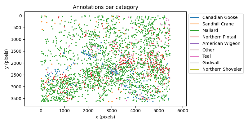
Let’s inspect how the annotations are distributed across the image coordinate system. We can color the centroid of each bounding box by the corresponding category to get a better sense of the distribution by species.

# We use a colormap of 10 discrete colours
# (we have 9 categories)
cmap = plt.cm.tab10

fig, ax = plt.subplots(figsize=(8, 4))

# Plot the centroids of the bounding boxes
sc = ax.scatter(
    ds.position.sel(space="x").values,
    ds.position.sel(space="y").values,
    s=3,
    c=ds.category.values,
    cmap=cmap,
)

# Add legend
# Note: we use ds.category.values rather than
# ds.map_category_to_str.values() because
# the array contains the padding value -1,
# which is also included in the scatter plot data.
legend_elements = [
    plt.Line2D([0], [0], color=cmap(i)) for i in np.unique(ds.category.values)
]
plt.legend(
    legend_elements,
    ds.map_category_to_str.values(),
    bbox_to_anchor=(1, 1),
    loc="best",
)
ax.set_title("Annotations per category")
ax.set_xlabel("x (pixels)")
ax.set_ylabel("y (pixels)")
ax.axis("equal")
ax.invert_yaxis()
plt.tight_layout()

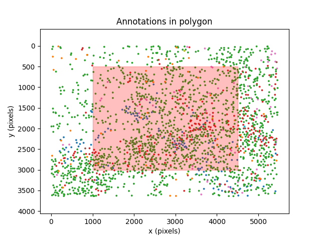
Count annotations within a region of interest

We may want to compute the number of annotations within a specific region of the image. We can do this using movement to define a movement.roi.PolygonOfInterest and then count how many annotations are within the polygon.

# Define a polygon
central_region = PolygonOfInterest(
    ((1000, 500), (1000, 3000), (4500, 3000), (4500, 500)),
    name="Central region",
)

# Plot all annotations
fig, ax = plt.subplots()
sc = ax.scatter(
    ds.position.sel(space="x").values,
    ds.position.sel(space="y").values,
    s=3,
    c=ds.category.values,
    cmap=cmap,
)
ax.set_title("Annotations in polygon")
ax.set_xlabel("x (pixels)")
ax.set_ylabel("y (pixels)")
ax.axis("equal")
ax.invert_yaxis()


# Plot ROI (region of interest) polygon on top
central_region.plot(ax, facecolor="red", edgecolor="red", alpha=0.25)

# Check the number of annotations in the polygon
# Note: if position is NaN, ``.contains_point`` returns ``False``
ds_in_region = central_region.contains_point(
    ds.position
)  # shape: (n_images, n_max_annotations_per_image)

n_annotations_in_region = ds_in_region.sum()
n_annotations_total = (~ds.position.isnull().any(axis=1)).sum()
fraction_in_region = n_annotations_in_region / n_annotations_total

print(f"Total annotations: {n_annotations_total.item()}")
print(f"Annotations in region: {n_annotations_in_region.item()}")
print(f"Fraction of annotations in region: {fraction_in_region * 100:.2f}%")

Total annotations: 2243
Annotations in region: 1155
Fraction of annotations in region: 51.49%

We can see that just over 50% of the annotations are within the region of interest defined by the polygon.

Transform dataset to a movement-like dataset

We can take further advantage of movement utilities by transforming our annotations dataset to a movement-like dataset.

To do this, we need to rename the dataset dimensions, add a confidence array, and add a time_unit attribute. We additionally rename the individuals coordinate values to follow the movement naming convention.

# Rename dimensions
ds_as_movement = ds.rename({"image_id": "time", "id": "individuals"})

# Rename 'individuals' coordinate values to be
ds_as_movement["individuals"] = [
    f"id_{i.item()}" for i in ds_as_movement.individuals.values
]

# Add confidence array with NaN values
ds_as_movement["confidence"] = xr.DataArray(
    np.full(
        (
            ds_as_movement.sizes["time"],
            ds_as_movement.sizes["individuals"],
        ),
        np.nan,
    ),
    dims=["time", "individuals"],
)

# Add time_unit attribute
ds_as_movement.attrs["time_unit"] = "frames"


print(ds_as_movement)
print(ds_as_movement.sizes)

<xarray.Dataset> Size: 433kB
Dimensions:      (time: 12, space: 2, individuals: 722)
Coordinates:
  * time         (time) int64 96B 0 1 2 3 4 5 6 7 8 9 10 11
  * space        (space) <U1 8B 'x' 'y'
  * individuals  (individuals) <U6 17kB 'id_0' 'id_1' ... 'id_720' 'id_721'
Data variables:
    position     (time, space, individuals) float64 139kB 4.493e+03 ... nan
    shape        (time, space, individuals) float64 139kB 95.0 43.0 ... nan nan
    image_shape  (time, space) int64 192B 5472 3648 5472 3648 ... 3648 5472 3648
    category     (time, individuals) int64 69kB 1 4 3 2 3 3 ... -1 -1 -1 -1 -1
    confidence   (time, individuals) float64 69kB nan nan nan ... nan nan nan
Attributes: (6)
Frozen({'time': 12, 'space': 2, 'individuals': 722})

Since this dataset represents manually labelled data, there isn’t really a confidence value associated with each of the annotations. Therefore, we add a confidence array with NaN values.

Similarly, we set the time unit to frames, but actually the images do not represent consecutive images in time. We do this to later be able to export the dataset in a movement-supported format that we can visualise in the movement napari plugin

Plot occupancy map using movement

We can now use the movement.plots.plot_occupancy() function to plot the occupancy map of the annotations. This is a two-dimensional histogram that shows for each bin the number of annotations that fall within it.

To determine the number of bins along each dimension, we use the aspect ratio of the images to define similarly sized bins. This makes the occupancy map more informative. Note that all images have the same dimensions.

# Determine aspect ratio of the images
image_width = np.unique(ds["image_shape"].sel(space="x").values).item()
image_height = np.unique(ds["image_shape"].sel(space="y").values).item()
image_AR = image_width / image_height

# Set number of bins along each dimension
n_bins_x = 75
n_bins_y = int(n_bins_x / image_AR)

# Plot occupancy map
fig, ax, hist = plot_occupancy(
    ds_as_movement.position,
    bins=[n_bins_x, n_bins_y],
)
fig.set_size_inches(10, 5)
ax.set_xlim(0, image_width)
ax.set_ylim(0, image_height)
ax.set_xlabel("x (pixels)")
ax.set_ylabel("y (pixels)")
ax.axis("equal")
ax.invert_yaxis()

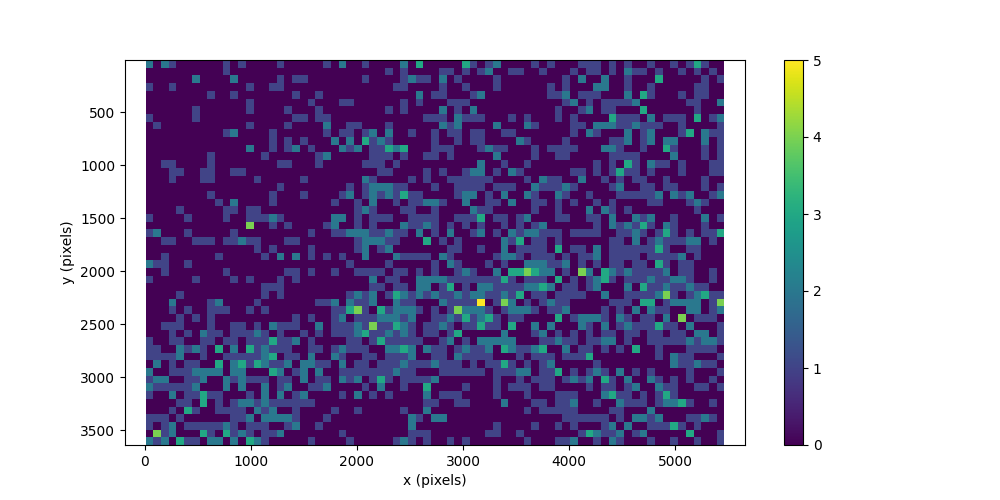
The occupancy map shows that the maximum count in each bin is 5 annotations, and the minimum count is 0 annotations. We can confirm this by inspecting the outputs of the movement.plots.plot_occupancy() function.

bin_size_x = np.diff(hist["xedges"])[0].item()
bin_size_y = np.diff(hist["yedges"])[0].item()

print(f"Bin size (pixels): ({bin_size_x}, {bin_size_y})")
print(f"Maximum bin count: {hist['counts'].max().item()}")
print(f"Minimum bin count: {hist['counts'].min().item()}")

Bin size (pixels): (72.77666666666667, 72.605)
Maximum bin count: 5.0
Minimum bin count: 0.0

Visualise the dataset in the movement napari plugin

We can export the movement-like dataset in a format that we can visualise in the movement napari plugin. For example, we can use the movement.io.save_bboxes.to_via_tracks_file() function, that saves bounding box movement datasets as VIA-tracks files.

save_bboxes.to_via_tracks_file(ds_as_movement, "waterfowl_dataset.csv")

PosixPath('waterfowl_dataset.csv')

You can now follow the movement napari guide to load the output VIA-tracks file into napari.

To visualise the annotations over the corresponding images, remember to first drag and drop the images directory into the napari canvas. You will find the images for the experts’ annotations under the data_dir / "experts" / "images" directory.

print(f"Images directory: {data_dir / 'experts' / 'images'}")

Images directory: /home/runner/.ethology/uas-imagery-of-migratory-waterfowl/experts/images

The view in napari should look something like this:

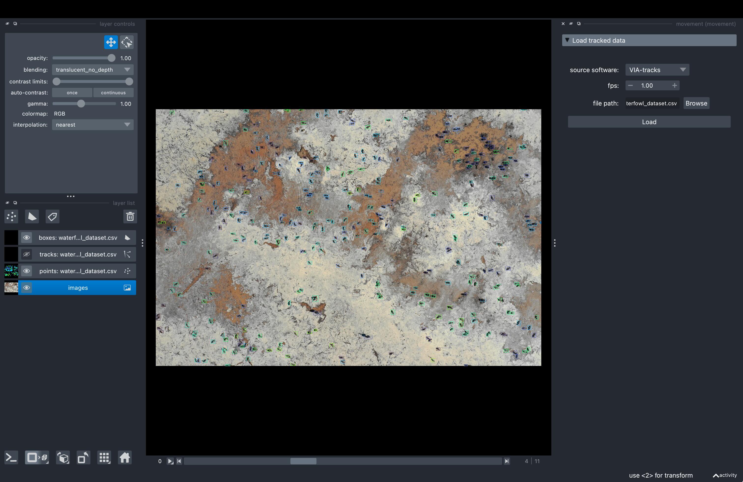
The bounding boxes are coloured by individual ID per image. Remember that the individual IDs are not consistent across images, so it makes more sense to hide the tracks layer for an easier visualisation, like in the example screenshot above.

Clean-up

To remove the output files we have just created, we can run the following code.

os.remove("waterfowl_dataset.csv")