Split an annotations dataset

Split an annotations dataset by grouping variable, and compare to random splitting.

This example demonstrates two dataset splitting strategies:

• Grouping-based split: splits the input dataset into two subsets with approximately the requested fractions, while keeping the values of a user-defined grouping variable (such as “videos” or “species”) entirely separate between subsets. We will explore two approaches: a group k-fold approach and an approximate subset-sum approach.

• Random split: splits the input dataset randomly into subsets with the requested fractions. It achieves precise split fractions but may mix values of variables across subsets (e.g., frames from the same video may be present in multiple subsets).

A grouping-based split is useful when defining a held-out test dataset with a specified percentage. For example, you may want to hold out ~10% of the annotated frames while ensuring that frames from the same video are not present in both the training and test sets.

In contrast, a random splitting strategy divides the dataset into precise proportions but does not prevent data leakage across subsets. This may be useful, for example, to generate multiple train/validation splits with very similar content for cross-validation.

Both approaches can be useful in different situations, and this example demonstrates how to apply them using ethology.

For more complex dataset splits, we recommend going through scikit-learn’s cross-validation functionalities, in particular the section on grouped data.

Imports

import sys
from collections import Counter
from pathlib import Path

import matplotlib.pyplot as plt
import numpy as np
import pooch
import xarray as xr
from loguru import logger

from ethology.datasets.split import (
    split_dataset_group_by,
    split_dataset_random,
)
from ethology.io.annotations import load_bboxes

# For interactive plots: install ipympl with `pip install ipympl` and uncomment
# the following line in your notebook
# %matplotlib widget

Configure logging for this example

By default, ethology outputs log messages to stderr. Here, we configure the logger to output logs to stdout as well, so that we can display the log messages produced in this example.

_ = logger.add(sys.stdout, level="INFO")

Download dataset

For this example, we will use the Australian Camera Trap Dataset which comprises images from camera traps across various sites in Victoria, Australia.

We use the pooch library to download the dataset to the .ethology cache directory.

data_source = {
    "url": "https://figshare.com/ndownloader/files/53674187",
    "hash": "4019bb11cd360d66d13d9309928195638adf83e95ddec7b0b23e693ec8c7c26b",
}

# Define cache directory
ethology_cache = Path.home() / ".ethology"
ethology_cache.mkdir(exist_ok=True)

# Download the dataset to the cache directory
extracted_files = pooch.retrieve(
    url=data_source["url"],
    known_hash=data_source["hash"],
    fname="ACTD_COCO_files.zip",
    path=ethology_cache,
    processor=pooch.Unzip(extract_dir=ethology_cache / "ACTD_COCO_files"),
)

print(*extracted_files, sep="\n")

/home/runner/.ethology/ACTD_COCO_files/3_Feral_animals_data_CCT.json
/home/runner/.ethology/ACTD_COCO_files/2_Region_specific_data_CCT.json
/home/runner/.ethology/ACTD_COCO_files/1_Terrestrial_group_data_CCT.json

Read as a single annotation dataset

The dataset contains three different COCO annotation files. We can load them as a single dataset using the ethology.io.annotations.load_bboxes.from_files() function.

ds_all = load_bboxes.from_files(extracted_files, format="COCO")

print(ds_all)
print(*ds_all.annotation_files, sep="\n")

<xarray.Dataset> Size: 10MB
Dimensions:      (image_id: 39426, space: 2, id: 6)
Coordinates:
  * image_id     (image_id) int64 315kB 0 1 2 3 4 ... 39422 39423 39424 39425
  * space        (space) <U1 8B 'x' 'y'
  * id           (id) int64 48B 0 1 2 3 4 5
Data variables:
    position     (image_id, space, id) float64 4MB 0.07955 nan nan ... nan nan
    shape        (image_id, space, id) float64 4MB 0.1591 nan nan ... nan nan
    image_shape  (image_id, space) int64 631kB 2048 1440 2048 ... 1152 2048 1152
    category     (image_id, id) int64 2MB 1 -1 -1 -1 -1 -1 ... 1 -1 -1 -1 -1 -1
Attributes: (5)
/home/runner/.ethology/ACTD_COCO_files/3_Feral_animals_data_CCT.json
/home/runner/.ethology/ACTD_COCO_files/2_Region_specific_data_CCT.json
/home/runner/.ethology/ACTD_COCO_files/1_Terrestrial_group_data_CCT.json

Inspect dataset

The combined dataset contains annotations for 39426 images, with each image having a maximum of 6 annotations. We can further inspect the different categories considered, the image sizes and the format of the image filenames.

# Categories
print("Categories:")
print(ds_all.map_category_to_str.values())
print("--------------------------------")

# Image sizes
print("Image sizes:")
print(np.unique(ds_all.image_shape.values, axis=0))
print("--------------------------------")

# Print a few image filenames
print("Sample image filenames:")
print(list(ds_all.map_image_id_to_filename.values())[0])
print(list(ds_all.map_image_id_to_filename.values())[30000])
print(list(ds_all.map_image_id_to_filename.values())[-1])

Categories:
dict_values(['animal', 'person'])
--------------------------------
Image sizes:
[[1920 1080]
 [2048 1152]
 [2048 1440]
 [2048 1536]
 [2560 1920]
 [2944 1656]
 [4000 3000]]
--------------------------------
Sample image filenames:
1_Terrestrial_group_classifier\Bird\Bird-0001.JPG
3_Feral_animals_data\Kangaroo\Kangaroo-0355.JPG
3_Feral_animals_data\Wallaby\Wallaby-1620.JPG

The image filenames encode a bit more of extra information, such as the original annotation file or the species class. We can use this to define possible grouping variables to split the images in the dataset.

Split by species: group k-fold approach

Let’s assume we want to split the dataset into two sets, such that each set has distinct species. This may be useful for example, if we want to evaluate the zero-shot performance of a species classifier, that is, its performance on species not seen during training. In this case we may want to split the dataset into train and test sets, while ensuring that no species are present in both train and test sets.

To do this, we first need to compute a variable that holds the species per image. Then we can split the images in the dataset based on the species they contain. Note that only one specie is defined per image.

We use a helper function to extract the information of interest from the image filenames.

# Helper function
def split_at_any_delimiter(text: str, delimiters: list[str]) -> list[str]:
    """Split a string at any of the specified delimiters if present."""
    for delimiter in delimiters:
        if delimiter in text:
            return text.split(delimiter)
    return [text]


# Get species name per image
species_per_image_id = np.array(
    [
        ds_all.map_image_id_to_filename[i].split("\\")[-2]
        for i in ds_all.image_id.values
    ]
)

# Add the species array to the dataset
ds_all["specie"] = xr.DataArray(
    species_per_image_id,
    dims="image_id",
)

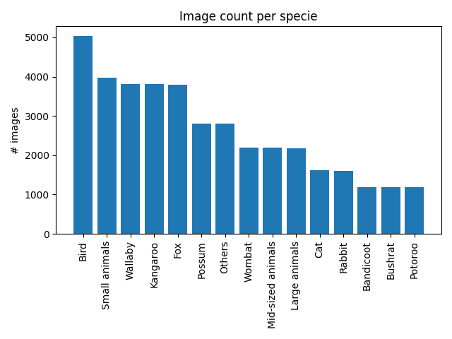
print(f"Total species: {len(np.unique(species_per_image_id))}")

Total species: 15

We have 15 different species in the dataset. With a bar plot we can visualise their distribution in the dataset.

count_per_specie = dict(Counter(ds_all["specie"].values).most_common())

fig, ax = plt.subplots()
ax.bar(
    count_per_specie.keys(),
    count_per_specie.values(),
)
ax.set_xticks(range(len(count_per_specie)))
ax.set_xticklabels(count_per_specie.keys(), rotation=90)
ax.set_ylabel("# images")
ax.set_title("Image count per specie")
plt.tight_layout()

We can now split the dataset by species using the ethology.datasets.split.split_dataset_group_by() function. For example, for a very specific 30/70 split, we would do:

fraction_1 = 0.3
fraction_2 = 1 - fraction_1

ds_species_1, ds_species_2 = split_dataset_group_by(
    ds_all,
    group_by_var="specie",
    list_fractions=[fraction_1, fraction_2],
)

2025-11-21 11:44:24.798 | INFO     | ethology.datasets.split:split_dataset_group_by:211 - Using group k-fold method with 3 folds and seed=42.

By default, the method parameter of the function is set to auto, which automatically selects the appropriate splitting method based on the number of unique groups and the requested split fractions. From the info messages logged to the terminal we can see that the automatically selected method was the “group k-fold” method. To force the use of this method, we can explicitly set the method parameter of the function to kfold.

We can check how close is the resulting split to the requested fractions, and verify that the subsets contain distinct species.

print(f"User specified fractions:{[fraction_1, fraction_2]}")

print(
    "Output split fractions: ["
    f"{len(ds_species_1.image_id.values) / len(ds_all.image_id.values):.3f}, "
    f"{len(ds_species_2.image_id.values) / len(ds_all.image_id.values):.3f}]"
)

print("--------------------------------")
print(f"Subset 1 species: {np.unique(ds_species_1.specie.values)}")
print(f"Subset 2 species: {np.unique(ds_species_2.specie.values)}")

User specified fractions:[0.3, 0.7]
Output split fractions: [0.336, 0.664]
--------------------------------
Subset 1 species: ['Bandicoot' 'Kangaroo' 'Possum' 'Rabbit' 'Wallaby']
Subset 2 species: ['Bird' 'Bushrat' 'Cat' 'Fox' 'Large animals' 'Mid-sized animals' 'Others'
 'Potoroo' 'Small animals' 'Wombat']

When using the “group k-fold” method, we can also generate different splits by setting a different value for the seed parameter. In the example below, we set the method parameter to kfold and use two different seed values, to generate two different splits.

# Split A with seed 42
ds_species_1a, ds_species_2a = split_dataset_group_by(
    ds_all,
    group_by_var="specie",
    list_fractions=[fraction_1, fraction_2],
    method="kfold",
    seed=42,
)

# Split B with seed 43
ds_species_1b, ds_species_2b = split_dataset_group_by(
    ds_all,
    group_by_var="specie",
    list_fractions=[fraction_1, fraction_2],
    method="kfold",
    seed=43,
)

2025-11-21 11:44:24.822 | INFO     | ethology.datasets.split:split_dataset_group_by:211 - Using group k-fold method with 3 folds and seed=42.
2025-11-21 11:44:24.840 | INFO     | ethology.datasets.split:split_dataset_group_by:211 - Using group k-fold method with 3 folds and seed=43.

We can verify that the split using the default value of the seed parameter (42) is the same as the first split computed above, but different from the split obtained with a different seed value (43). The output fractions in both cases are approximately the requested fractions.

print(
    "Output split fractions for seed 42: ["
    f"{len(ds_species_1a.image_id.values) / len(ds_all.image_id.values):.3f}, "
    f"{len(ds_species_2a.image_id.values) / len(ds_all.image_id.values):.3f}]"
)

print(
    "Output split fractions for seed 43: ["
    f"{len(ds_species_1b.image_id.values) / len(ds_all.image_id.values):.3f}, "
    f"{len(ds_species_2b.image_id.values) / len(ds_all.image_id.values):.3f}]"
)


assert ds_species_1a.equals(ds_species_1)
assert ds_species_2a.equals(ds_species_2)
assert not ds_species_1a.equals(ds_species_1b)
assert not ds_species_2a.equals(ds_species_2b)

Output split fractions for seed 42: [0.336, 0.664]
Output split fractions for seed 43: [0.365, 0.635]

We have mentioned that by default, the method in the ethology.datasets.split.split_dataset_group_by() function is set to auto, which automatically selects the appropriate method based on the number of unique groups and the requested number of folds. The number of required folds is calculated as the closest integer to 1 / min(list_fractions).

In this case, we have 15 unique species, and 1/0.3 ~ 3 folds. Since there are more unique groups than folds, the the auto setting defers to the preferred “group k-fold” method. The “group k-fold” method is preferred because it allows us to compute different disjoint splits for the same requested fractions via the seed parameter.

If the number of unique groups is less than the requested number of folds, the auto setting defers to approximate subset sum algorithm. to compute a solution. We explore this case in the next section.

Split by input annotation file: approximate subset-sum approach

Let’s consider another case, in which we would like to split the images in the dataset by the annotation file they come from.

As before, we first compute the annotation file per image, which we derive from the image filename. Then we add the annotation file array to the dataset.

# Get annotation file per image
annotation_file_per_image_id = np.array(
    [
        split_at_any_delimiter(
            ds_all.map_image_id_to_filename[i],
            ["\\"],
        )[0]
        for i in ds_all.image_id.values
    ]
)

# Add to dataset
ds_all["json_file"] = xr.DataArray(
    annotation_file_per_image_id, dims="image_id"
)

We can now split the dataset by annotation file using the ethology.datasets.split.split_dataset_group_by() function with the method parameter set to apss (approximate subset-sum).

ds_annotations_1, ds_annotations_2 = split_dataset_group_by(
    ds_all,
    group_by_var="json_file",
    list_fractions=[fraction_1, fraction_2],
    method="apss",
)

2025-11-21 11:44:26.102 | INFO     | ethology.datasets.split:split_dataset_group_by:219 - Using approximate subset-sum method with epsilon=0.

The log message confirms we have used the “approximate subset-sum” method. It also mentions an epsilon parameter, which is optional. This is the percentage of the optimal solution that the solution is guaranteed to be within. If epsilon is 0 (default), the solution will be the best solution (optimal) for the requested fraction and grouping variable.

The algorithm computes the smallest subset to be less than or equal to the smallest requested fraction.

print(f"User specified fractions:{[fraction_1, fraction_2]}")

output_fractions = [
    len(ds_annotations_1.image_id.values) / len(ds_all.image_id.values),
    len(ds_annotations_2.image_id.values) / len(ds_all.image_id.values),
]
print(f"Output split fractions for epsilon 0: {output_fractions}")

print(f"Subset 1 files: {np.unique(ds_annotations_1.json_file.values)}")
print(f"Subset 2 files: {np.unique(ds_annotations_2.json_file.values)}")

User specified fractions:[0.3, 0.7]
Output split fractions for epsilon 0: [0.18130167909501343, 0.8186983209049865]
Subset 1 files: ['2_Region_specific_data']
Subset 2 files: ['1_Terrestrial_group_classifier' '3_Feral_animals_data']

We can verify that the subsets contain distinct annotation files. Since we used the default epsilon=0, this split is the best solution we can get within the specified constraints. In this case there are only three possible splits of the dataset, since there are only three possible values for the source annotation file.

The choice of epsilon involves a trade-off between accuracy and speed. In more cases with many possible splits, we may want to use a larger epsilon value, to get faster to a solution that is close enough to the optimal one.

Split using random sampling

Very often we want to compute splits for a specific fraction, and don’t care if a grouping variable (such as “species” or “source annotation file”) is mixed across subsets.

In this case, we can use random sampling with the function ethology.datasets.split.split_dataset_random(). This function shuffles the dataset and then partitions it according to the specified fractions. By setting a different value for the seed, we can again get different splits for the same requested fractions.

ds_species_1, ds_species_2 = split_dataset_random(
    ds_all,
    list_fractions=[fraction_1, fraction_2],
    seed=42,
)


print(f"User specified fractions:{[fraction_1, fraction_2]}")

print("Split fractions:")
print(len(ds_species_1.image_id.values) / len(ds_all.image_id.values))
print(len(ds_species_2.image_id.values) / len(ds_all.image_id.values))

User specified fractions:[0.3, 0.7]
Split fractions:
0.2999797088215898
0.7000202911784101